Treasure Hunting 2
Conditional Poisson Stochastic Beam Search
Today I’m going to introduce the paper ‘Conditional Poisson Stochastic Beam Search’ by Clara Meister, Afra Amini, Tim Viera, and Ryan Cotterell, you can find the paper [here]
And different from the previous ‘Treasure Hunting’ episodes, in this very episode, instead of introducing the paper following its structure, I re-arrange the paper and introduce it in a more logical way that I consider myself better to understand. (And to be honest the paper is really tough for me !) Though still some parts of the paper remain unclear for me, I try my best to illustrate its main ideas.
Note that: ‘xxx’ means quoted from the paper; xxx is to underline; sub_title is the sub title I named to help understand the structure of the paper; ‘xxx’ is the question / comments I raised to help understand the idea/logic of the paper; And the formulas are all from the paper (some minor modification for consistence with my own signs are done), and for writing fluency, I sometimes introduce concepts as ‘We define …’ instead of ‘The authors define …’
Deterministic vs. Stochastic
- What is beam search ?
Beam search is a very important decoding strategy for NLP tasks involving generation (e.g., NMT, text generation), they’re usually done in the following way:
For example, we’re going to generate a sentence with a vocabulary $\mathcal{V}=\{I, like, spring, EOS\}$, where $BOS$ only indicates the end of the sentence. At the beginning of generation, we start with a $BOS$ token which indicates the beginning of the sentence. And beam search aims to find the top-$K$ possible decoding options at each time step, thus, at step 1, we may have a probability of ${I=0.6, like=0.1, spring=0.3}$, indicating the likelihood of a word from $\mathcal{V}$ being placed at the step ( at step 1, which means after $BOS$), and let the $K=2$ , then the decoding process can be roughly illustrated as:
Where ‘$+$’ means appending the word after the sequence from previous step, and for simplicity $BOS$ is removed after step 1. And we can see that each step the preserved top-$K$ beams (with highest top-$K$ probability of being generated, marked red) will have a possible extension over $\mathcal{V}$, generating $K\times |\mathcal{V}|$ candidates, and then top-$K$ high probability beams are selected then (in above case, at step 2, they are: ‘I like’ and ‘spring like’).
- What’s the drawbacks of beam search ? And can we solve them ?
With the above brief introduction about beam search, now we face a very tough question: What if the $K+1$-th beam at step $t$ is actually a better beam at step $t+1$ ? That means, by deterministically select top-$K$ best options out of $K\times |\mathcal{V}|$ at each time step, we may lose some better candidates ! And we of course want a generalized version of beam search, which can include beam search as a special case while has some stochasticity. $\longrightarrow$ and this leads to the answer: by sampling ! Instead of deterministically choose top-$K$ beams at each time step, we stochastically sample a set with $K$ beams out of a base set with $K\times |\mathcal{V}|$ beams, and of cause a set with top-$K$ beams (in this sense, it means beam search) will still have a probability being sampled, thus we can say the stochastic sampling strategy is the generation of the deterministic beam search.
- How the problem is formed ?
And the authors formulate the beam search problem as follows:
the generation process can be written as:
‘where $\textbf{y}$ is a member of a set of well-formed outputs $\mathcal{Y}$ ‘. And $\textbf{y}=\{y_1,\,y_2,\,… \}$ where $y_k \in \mathcal{Y}$, $\textbf{y}_{< t}=\{y_1,\,y_2,\,…,y_{t-1},\,y_t\}$. And in the following discussion, a max generation length $T$ for the sentence is considered.
To solve the problem of $\textbf{y}^{*}=\underset{y\in \mathcal{Y}}{argmax}\,\,log\,p(\textbf{y})$, the beam search is then formulated as:
\[\begin{eqnarray*} Y_0 &=& {BOS} \tag{1} \\ Y_t &=& \underset{Y_t^{'}\subseteq B_t}{argmax}\,\,Q_t({Y_t^{'}}\,\|\,Y_{t-1}) \tag{2} \\ re&turn\,Y_T \end{eqnarray*}\]Where:
Note that $Q_t(Y_t\,|\,Y_{t-1})$ is only assigned value when $|Y_t|=K$, and the though the assigned value is written as $\prod \limits_{n=1}^{N}w_n$ , it actually means for those $w_n$’s belonging to the set $Y_t$ . For example, if $K=3,\,N=9$ and ${w_1,\,w_4,\,w_5}$ belongs to $Y_t$ , then $\prod \limits_{n=1}^{N}w_n$ indicates $w_1\times w_4\times w_5$ .
And now let’s continue to sort out some undefined concepts:
if we define steps as $t=1,\,2,\,…T$, and $Y_{t-1}\,\circ\,V\overset{def}{=}{\textbf{y}\,\circ\,y\,|\,\textbf{y}\in Y_{t-1}\,\,\textbf{and}\,\,y\in V}$ , where $\circ$ means concatenation (which is the ‘$+$’ in the above-mentioned case ), and also: $B_t\overset{def}{=}Y_{t-1}\,\circ\,V$, thus $B_t$ is actually: ${\textbf{y}_{\leq t}^{(1)},\,…\textbf{y}_{\leq t}^{(N)}}$ where $N=K\times |\mathcal{V}|$ (except when $t=0$ since there is only a choice of $|\mathcal{V}|$ words for $BOS$), again for simplicity, ${\textbf{y}_{\leq t}^{(1)},\,…\textbf{y}_{\leq t}^{(N)}}$ is represented as ${1,\,2,\,…N}$ . And $w_n\,(=p(\textbf{y}_{\leq t}^{(n)}))$ indicates the probability of generation under the model (e.g., $spring+like={\color{red}0.3\times 0.8}$)
Conditional Poisson Stochastic Beams
- why called ‘conditional Poisson stochastic beam search’ ?
With the above mentioned definitions, a normalization to ‘the time-step dependent set function’ $Q_t(Y_t\,|\,Y_{t-1})$ (which makes it a distribution) can derive the ‘sample-without-replacement’ (‘without-replacement’ means one element after being chosen, can’t be chosen again) version of beam search:
And ‘This recursion corresponds to performing conditional Poisson sampling (CPS; Hájek 1964;see App. A for overview), a common sampling-without-replacement design (Tillé, 2006)3, at every time step.’ where in 3 the authors explain: ‘A sampling design is a probability distribution over sets of samples.’ And that’s why the proposed work is referred to as ‘conditional Poisson stochastic beam search’ (CPSBS)
- How is it performed in detail ?
First of all, to understand the probability of a size $K$ set $Y_T$ is sampled, its marginal probability can be written as follows:
And the summation is actually computing the marginal distribution out of a joint distribution. The above marginal distribution tells us that: for the final beam set $Y_T$ of size $K$, there’re roughly (less than): $|\text{#}Y_1|\times |\text{#}Y_2|\times ··· \times |\text{#}Y_{T-1}| \times |\text{#}Y_T|$ available values to be assigned with, where $|\text{#}Y_t|$ denotes the number of possible values for set $Y_t$ at time-step $t$ . And the authors state that: ‘Note the structural zeros of $Q_t$ prevent any incompatible sequence of beams’ , which can be answered by the following example:
For a $K=2$ CPSBS with a vocabulary $\mathcal{V}={1,\,2,\,…\,,7}$ . If at $t=1$ , $Y_1$ can be: ${BOS+1,\,BOS+3}$ , then at $t=2$, $Y_2$ can be: ${BOS+12,\,BOS+15,\,BOS+32,\,BOS+34}$ .
However, note that $Q_2(Y_2=BOS+12\,|\,Y_1=BOS+3)$ and $Q_2(Y_2=BOS+15\,|\,Y_1=BOS+3)$ are both incompatible, vice versa. And this explains why $Q_t=0$ can prevent ‘incompatible sequence of beams’ and why the assignable values are less than the multiplication of available values at each time step.
And also, for a given $Y_T^{(m)}=\{\textbf{y}_{\leq T}^{(m_1)}\,,\,\textbf{y}_{\leq T}^{(m_2)}\,,\,…,\,\textbf{y}_{\leq T}^{(m_K)}\}$, it’s generation probability can be simply computed as (no need to compute the summation, since the stochastic sample at each time-step should be deterministic in order to generate $Y_T^{(m)}$, to be specific, it means only $BOS+1$ can generate $BOS+12$ and $BOS+15$) : $P(Y_T=Y_T^{(m)})\,=\prod \limits_{t=1}^{T}Q_t\,(\,Y_t=\{\textbf{y}_{\leq t}^{(m_1)}\,,\,\textbf{y}_{\leq t}^{(m_2)}\,,\,…,\,\textbf{y}_{\leq t}^{(m_K)}\}\,|\,Y_{t-1}=\{\textbf{y}_{\leq t-1}^{(m_1)}\,,\,\textbf{y}_{\leq t-1}^{(m_2)}\,,\,…,\,\textbf{y}_{\leq t-1}^{(m_K)}\})$
Thus, for a given final beam set $Y_T^{(m)}$ , we can actually compute its generation probability.
- How is CPSBS performed ?
Now we formally look deeper into how CPSBS is performed at time-step $t$ . Before we start, bear in mind that we have a few things to do to perform CPSBS: 1. the previous set function $Q_t(Y_t\,|\,Y_{t-1})$ is a scoring function (see here), we need to convert it into a distribution to perform sampling; 2. an efficient and general algorithm should be there for us to perform sampling at each time-step; With these two preliminaries acknowledged, we now see how CPSBS is performed by the authors:
Step 1: Normalize $Q_t(·\,|\,Y_{t-1})$ .
We know that now $Q_t(·\,|\,Y_{t-1})$ should be able to sample a $Y_t^{any}$ containing $K$ beams based on the previous size-$K$ set $Y_{t-1}$ , and since we are actually selecting $K$ beams out of $N=K \times |\mathcal{V}|$ , there are actually $\binom{N}{K}$ options for us to sample such a size-$K$ set $Y_t^{any}$ , thus, $p(Y_t^{any})$ should be modified by the summation of the probabilities of size-$K$ sets that are possible to be sampled, and the normalization constant is defined as:
Where the notation $\prod \limits_{n=1}^{N}w_n$ still follows the meaning of this . And following Kulesza and Taskar (2012, see here), an iterative algorithm can be proposed: ( For detailed pseudocode please refer to the App. C of the paper)
And $Z_t=W\binom{N}{K}$.
Step 2: Sample from $Q_t(·\,|\,Y_{t-1})$ (normalized) .
After the distribution $Q_t(·\,|\,Y_{t-1})$ is normalized, the following algorithm is proposed by the authors:
1: $Y_t \longleftarrow \emptyset$ (Initialization)
2: for$\,\,n=N,\,…\,,1$ :
$\qquad k\longleftarrow K-|Y_t|$ (Number of remaining elements)
Add the $n^{th}$ element of $B_t$ to $Y_t$ with probability:
$\frac{w_n\,W\binom{n-1}{k-1}}{W\binom{n}{k}}$
3: return $Y_t$ (Guaranteed to have size $K$)
And I explain the why the probability is $\frac{w_n\,W\binom{n-1}{k-1}}{W\binom{n}{k}}$ and why it is guaranteed to have size $K$ as follows:
why the probability is $\frac{w_n\,W\binom{n-1}{k-1}}{W\binom{n}{k}}$ ?
We can consider $\frac{w_n\,W\binom{n-1}{k-1}}{W\binom{n}{k}}$ as the probability of the $n^{th}$ element of $B_t$ being included in the final $Y_t$ . With (8) , we can derive:
Where we consider $\frac{W\binom{n-1}{k}}{W\binom{n}{k}}$ as the probability of the $n^{th}$ element of $B_t$ being excluded in the final $Y_t$ . And according (7) and (8), we can interpret $W\binom{n}{k}$ as the total probability of choosing the remaining $k$ of the total $K$-to-be-chosen elements out of the available element set : ${n,\,n-1,\,…\,1}$, and since the elements are chosen in a reverse order (from $N$ to $1$), thus $W\binom{n-1}{k}$ is then the total probability of choosing the remaining $k$ of the total $K$-to-be-chosen elements out of the available element set : ${n-1,\,…\,1}$ where element $n$ is excluded. Thus, the probability of the $n^{th}$ element of $B_t$ being excluded in the final $Y_t$ is: probability of choosing $k$ elements without element $n$ / probability of choosing $k$ elements considering element $n$ (though it may not be necessarily chosen), which is: $\frac{W\binom{n-1}{k}}{W\binom{n}{k}}$ .
why it is guaranteed to have size $K$ ?
Let’s consider an extreme situation: for the first $N-K$ elements, namely ${N,\,…\,,K+1}$, no elements are added to $Y_t$ , and now $n=k\,(=K)$, in this sense, according to (8), the next element $K$, is added with a probability $\frac{w_n\,W\binom{n-1}{k-1}}{W\binom{n}{k}}=1-\frac{W\binom{n-1}{k}}{W\binom{n}{k}}$ ( though this only holds when $k\in (0,\,n)$ ) where $W\binom{n}{k}=1$ and $W\binom{n-1}{k}=0$, thus, with a deterministic probability ‘1’ , the element $n$ will then be added, and $n,\,k$ again equals $K-1$, which means the above selecting process goes on again until all the remaining elements are added.
Statistical Estimation with CPSBS
- A supplementary: what is inclusion probability ?
For a certain beam $\textbf{y}_{\leq t}^{(n)}$ at time-step $t$, what’s its probability of being included in the $Y_t$ of this time-step? (i.e., $Pr(\textbf{y}_{\leq t}^{(n)}\in Y_t)$, which is called the inclusion probability) To understand this, we denote the inclusion probability of $\textbf{y}_{\leq t}^{(n)}$ ( w.r.t. $Q_t(·\,|\,Y_{t-1})$ ) as :
Where $Y_t$ ranges over all the possible size-$K$ set sampled from the base set $B_t$ , and $\mathbb{1}(\textbf{y}_{\leq t}^{(n)}\in Y_t)$ is an indicator, equals one if the desired beam $\textbf{y}_{\leq t}^{(n)}$ is in $Y_t$ , zero otherwise. And if at time-step $t$ we choose $w_n$ to make $\pi_{Q_t}(\textbf{y}_{\leq t}^{(n)}\,|\,Y_{t-1})\approx p(\textbf{y}_{\leq t}^{(n)})$ . It can recover beam search as we anneal the chosen weights: $w_n\rightarrow w_n^{1/\tau}$ as $\tau \rightarrow 0$, and the conditional Poisson distribution will assign probability 1 to the set containing the top-$K$ beams at time-step $t$ . And finding such $w_n$ s resulting a desired inclusion probability is possible, though requires solving a numerical optimization problem (Aires, 1999 {see [paper]}; Grafström, 2009 {see [paper]}) , thus the authors use an approximation of $w_n=p(\textbf{y}_{\leq t}^{(n)})/(1-p(\textbf{y}_{\leq t}^{(n)}))$ which yields good approximation in both theory and practice as reported in (Hájek, 1981 {see [[paper]]}; Bondesson et al. {see [paper]}, 2006; Aires, 1999 {see [paper]}) .
- How do we estimate statistical features of CPSBS ?
With above-mentioned sampling process of CPSBS at each time-step known, now we of course can’t help thinking about some questions like: ‘How to calculate one specific beam, say: $\textbf{y}^{(m)}$’s entropy ?’ or ‘How do we compute the BLEU score (see BLEU) of $\textbf{y}^{(m)}$ ?’ . And unlike beam search where $\textbf{y}^{(m)}$ appears deterministically, in CPSBS, $\textbf{y}^{(m)}$ can be in many different $Y_T$ s, which leads us to the statistical estimation of the CPSBS. In a more mathematical way, as the authors state: ‘Let be $f:\,\mathcal{Y}\rightarrow \mathbb{R}^{d}$ , we seek to approximate its expected value under $p$:’
And a traditional way is the Monte Carlo estimator: $G_{MC}\overset{def}{=}\frac{1}{M}\sum_{m=1}^{M}f(\textbf{y}^{(m)})$ where $\textbf{y}^{(m)}\overset{i.i.d}{\sim}p$ , and the authors argue that: ‘However, in the special case of sampling from a finite population—which is extremely common in NLP—it can be very wasteful. For example, if a distribution is very peaked, it will sample the same item repeatedly; this could lead to inaccurate approximations for some $f$. As a consequence, the mean square error (MSE) of the estimator with respect to $\mathbb{E}_{\textbf{y}\sim p}[f(\textbf{y})]$ can be quite high for small M.’ And since the sampling process of CPSBS is not independent (which means $\textbf{y}\nsim p$) , a Horvitz–Thompson estimator (see [paper] here) is used to estimate the expectation of a certain $f$ over $Y_T\sim P$ , where $P$ is this :
- Estimate the inclusion probability $\pi_P(y)$
As equation (11) mentions, to use the Horvitz–Thompson estimator we need to know the probability of generation: $p(y)$ (which is rather easy since it simply equals that of $Y_T$) and the inclusion probability: $\pi_P(y)$ . However, though computing $\pi_P(y)$ can give us an ‘unbiased’ HT estimator (for detailed information please refer to App. B. of the paper), to actually compute such a value is almost impossible (see the summations in the following equation). And of course, we have two ways: Naive Monte Carlo and Importance sampling to estimate the following inclusion probability:
The Naive Monte Carlo estimator:
We can defined the Naive Monte Carlo estimator as follows:
Where $Y^{(m)}\sim P$ . And ‘$\hat{\pi}_p^{MC}$ is an unbiased estimator of $\pi_P$ with variance : $\mathbb{V}[\hat{\pi}_P^{MC}]=\frac{1}{M}(\pi_P(\textbf{y})-\pi_P(\textbf{y})^{2})$ . Meanwhile $1/\hat{\pi}_P^{MC}$ is a consistent estimator of $1/\pi_P$ with asymptotic variance : $\mathbb{V}_a[\frac{1}{\hat{\pi}_P^{MC}}]=\frac{1}{M}(\frac{1}{\pi_P(\textbf{y})^{3}}-\frac{1}{\pi_P(\textbf{y})^{2}})$’ . (for proof please refer to the App. B.2. of the paper)
And we can easily see the problems of the Naive Monte Carlo estimator. For a desired beam $\textbf{y}$ with a very low $\pi_P(\textbf{y})$ , the asymptotic variance of its estimated reverse is very high, thus resulting a less accurate estimate. Also, consider the summation in (13) , most of the sampled $Y_T^{(m)}$ s may not contain the desired beam $\textbf{y}$ , thus the sampling process will be time-consuming in order to have one $Y_T^{(m)}$ contain the desired beam $\textbf{y}$ , and most cases are the estimate of rare desired beam $\textbf{y}$ s tend to be zero.
Importance sampling:
To solve the problem of sampling lots of $Y_T^{(m)}$ s to contain the desired beam $\textbf{y}$ . We can actually make the sampled set include the desired beam $\textbf{y}$ , which the authors call: hindsight samples : $\tilde{Y}_1,\,\tilde{Y}_2,\,…,\tilde{Y}_T$ where they all contain the desired beam $\textbf{y}$ . And the hindsight samples can be generated through a proposal distribution conditioned on $\textbf{y}$ :
And according to the authors, the proposal distribution can be done by a simply modification to the CPSBS algorithm: ‘where $w(\textbf{y})$ corresponding to $\textbf{y}_{\leq t}^{(n)}$ is plcaed at the beginning and added to $Y_t$ deterministically’. For simplicity, the fact $\tilde{Y}$ and $\tilde{Q}$ are conditioned on $\textbf{y}$ are omitted. And the following lemma is proposed by the authors (see the proof in the App. B.2. of the paper):
Where $\tilde{P}(\tilde{Y}_1,\,…,\tilde{Y}_T)\overset{def}{=}\prod \limits_{t=1}^{T}\tilde{Q}_t(\tilde{Y}_t\,|\,\tilde{Y}_{t-1})$ is the joint proposal distribution . And $P(\tilde{Y}_1,\,…,\tilde{Y}_T)\overset{def}{=}\prod \limits_{t=1}^{T}Q_t(\tilde{Y}_t\,|\,\tilde{Y}_{t-1})$ is defined as the joint probability of the beams under the original distribution $Q_t$ . And both $P$ and $\tilde{P}$ conditioning on $Y_0$ are omitted.
And the computation for (15) makes use of the fact that the inclusion probability $\pi_{Q_t}(\textbf{y}_{\leq t})$ for a given $Q_t$ at each time-step can be computed with dynamic programming: (see the pseudocode in App. C. of the paper)
Where $\textbf{y}_{\leq t}^{(n)}$ indicates the $n$-th candidate beam out of the $N$ beams. And for $\tilde{Y}_T^{(m)}\sim \tilde{P}$ where $\tilde{P}$ is defined by the proposal distribution in (14) . The inclusion probability in the HT estimator mentioned in (11) can be estimated as:
And the above estimation can be derived from:
Which indicates that (17) inherits unbiasedness from the Naive Monte Carlo estimator in (13) . And the following properties can be observed from the Importance Sampling strategy in (17) :
‘$\hat{\pi}_p^{IS}$ is an unbiased estimator of $\pi_P$ . Meanwhile $1/\hat{\pi}_P^{IS}$ is a consistent estimator of $1/\pi_P$ with an upper bound on asymptotic variance : $\mathbb{V}_a[\frac{1}{\hat{\pi}_P^{MC}}]\leq\frac{1}{M}\frac{r-1}{\pi_P(\textbf{y})^{2}}$ where an assumption that “for all $\tilde{Y}_1,\,…\,,\tilde{Y}_T$ the following bound: $\frac{\prod \limits_{t=1}^{T}\pi_{Q_t}(\textbf{y}_{\leq t}\,|\,\tilde{Y}_{t-1})}{\pi_P(\textbf{y})}\leq r$ holds” is made’ (for proof please refer to the App. B.2. of the paper). And the authors also mention that when $\prod \limits_{t=1}^{T}\pi_{Q_t}(\textbf{y}_{\leq t}\,|\,\tilde{Y}_{t-1})$ approximates the real $\pi_P(\textbf{y})$ , the variance of the Importance Sampling estimate is relatively smaller that that of the Naive Monte Carlo, ‘which is often the case for estimators when a proposal distribution is chosen judiciously (Rubinstein and Kroese, 2016).’ (see [paper])
Experiments
To test the performance of CPSBS and its HT estimator, they are tested on the sentence-level BLEU together with the Monte Carlo estimator, Sum and Sample estimator, an estimator for Stochastic Beam Search. To observe behaviors of the HT estimator under both high- and low-entropy setting, the model’s distribution is annealed as: $p_\tau(y_t\,|\,\textbf{y}_{<t})\propto p\,(y_t\,|\,\textbf{y}_{<t})^{\frac{1}{\tau}}$ .
- Additional estimators to be compared with
For Monte Carlo sampling strategy with sample size $K$, the estimator: $G_{MC}\overset{def}{=}\frac{1}{M}\sum_{m=1}^{M}f(\textbf{y}^{(m)})$ is used to estimate the expectation of $f$ under the model where: $\textbf{y}^{(1)},\,…\,,\textbf{y}^{(K)}\overset{i.i.d.}{\sim}p$ . And this estimator is also used as a baseline by computing 50 times with a sample size of 200 each time.
For Sum and Sample, the sum-and-sample estimator is an unbiased estimator which takes { a deterministically chosen set $Y$ of size $K-1$ (obtained using beam search in this experiment) and a sampled $\textbf{y}^{‘}$ from the remaining set $supp(p)\backslash Y$ } as input, the estimator can be written as : $G_{SAS}\overset{def}{=}\sum_{k=1}^{K-1}p(\textbf{y}^{(k)})f(\textbf{y}^{(k)})+\left( 1-\sum_{k=1}^{K-1}p(\textbf{y}^{(k)})\right)f(\textbf{y}^{‘})$ .
For Stochastic Beam Search, which is a similar Sample-Without-Replacement algorithm built on the beam search making use of the truncated Gumbel random variables at each time-step. And a estimator following the Horvitz-Thompson scheme is built (similar to (11)).
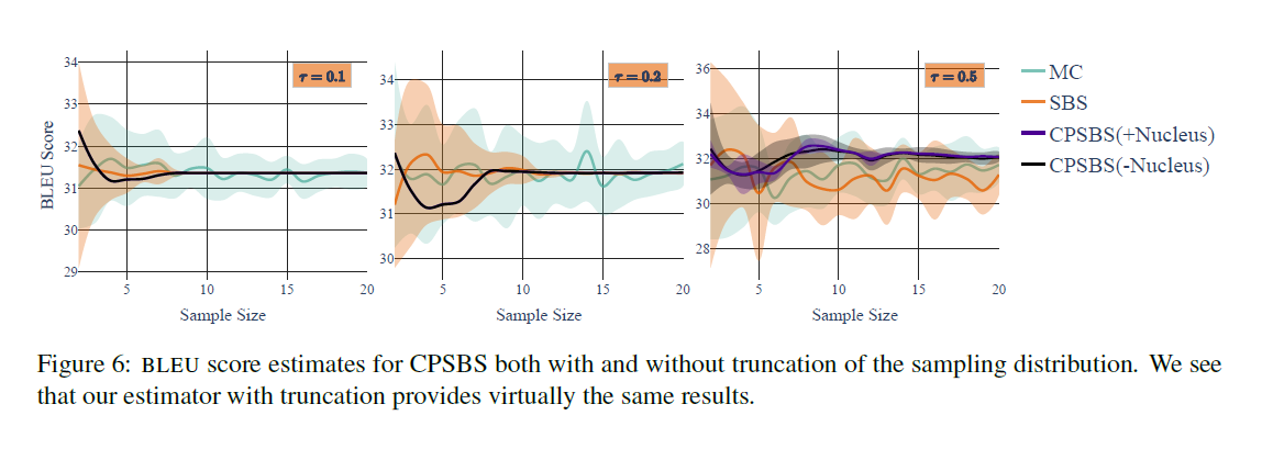
And for a more efficient estimation, a truncated distribution is used which preserves the 99% of the probability mass to accelerate the computation of (7), which is ‘similar to the process in nucleus sampling (Holtzman et al., 2020)’ (see [paper] here). See the differences here:
- the function $f$ s whose expectation is to be computed
BLEU score estimation:
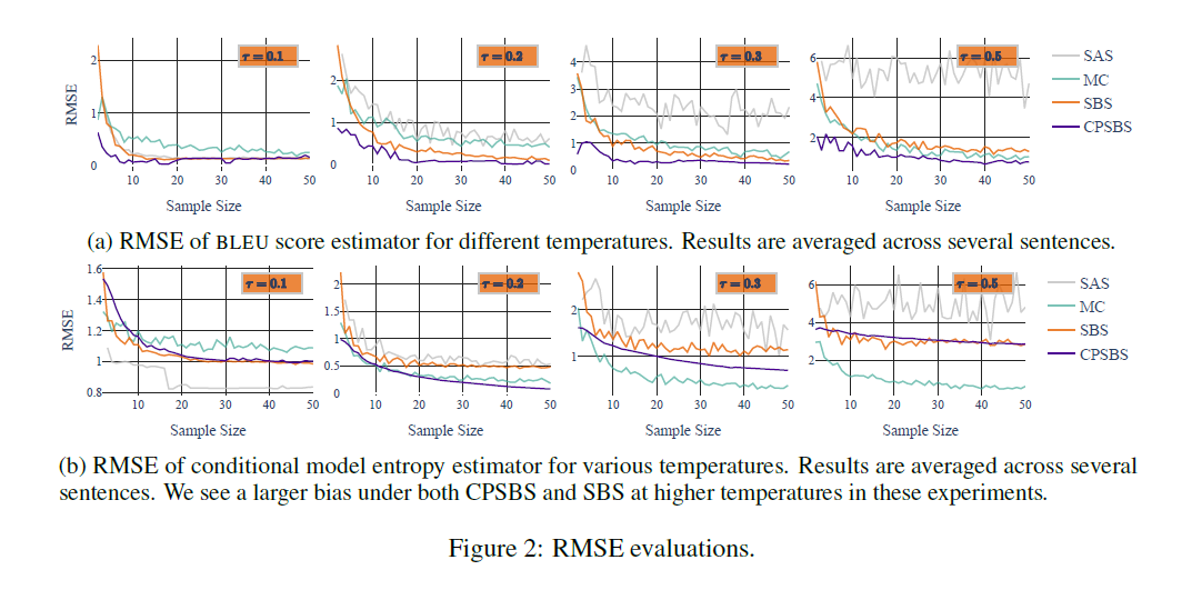
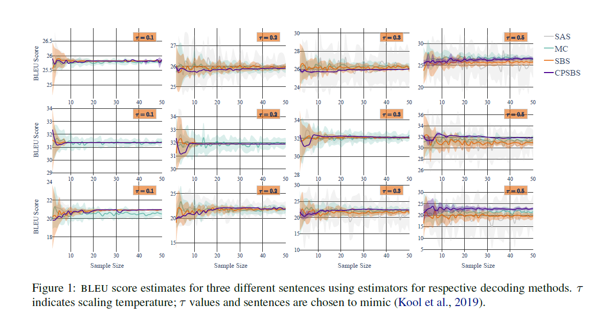
the score is defined as : $f(\textbf{y})=BLEU(\textbf{x},\,\textbf{y})$ where if for NMT models, $\textbf{x}$ is the reference translation. The sampling process is repeated 20 times and the mean and variance are plotted for each sample size. And see in Figure 2.a about the RMSE of the BLUE estimators that when temperature is not relatively high, CPSBS has a quite low RMSE, when the temperature is high, CPSBS becomes biased, which is ‘similar to Kool et al. (2019)’s observations’ (see [paper] here).
Conditional Entropy Estimation:
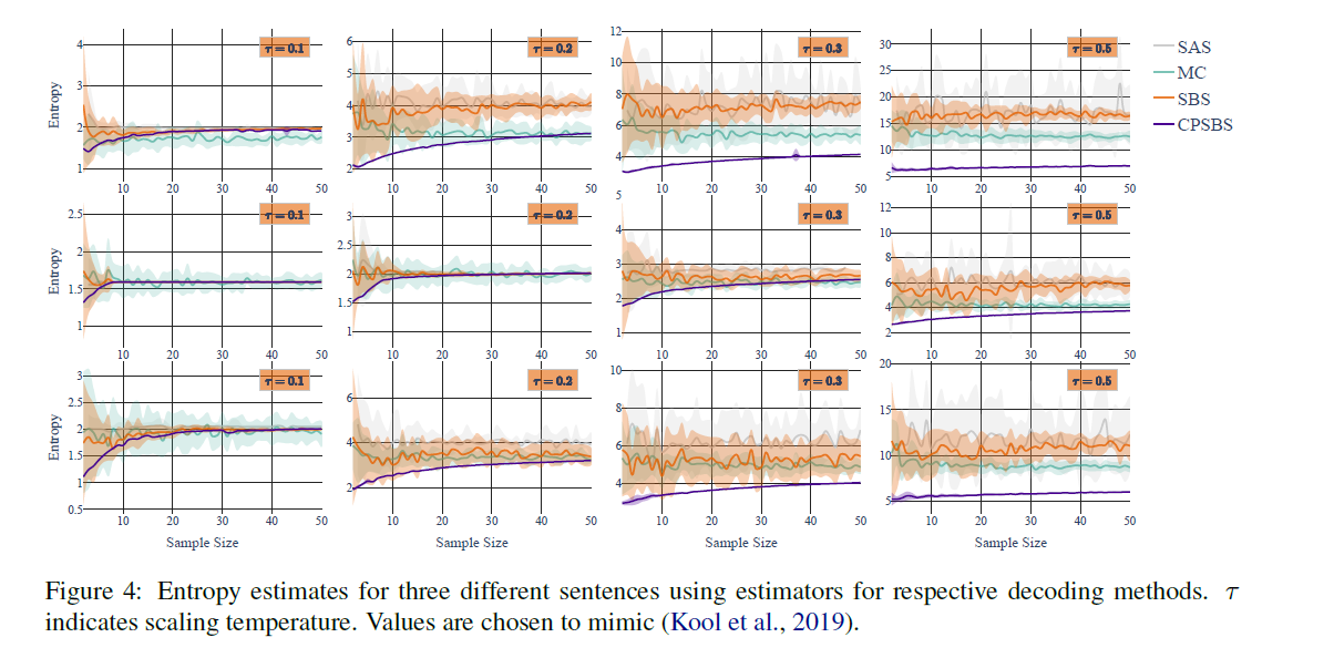
To estimate a model’s conditional entropy: $f(\textbf{y})=-log\,p(\textbf{y}\,|\,\textbf{x})$ where $\textbf{x}$ can be seen as the initial information necessary to generate the first set of beams, i.e., $Y_1$ . And see in Figure 2.b to see the RMSE for the conditional entropy estimation.
RMSE:
The RMSE evaluations for above-mentioned BLUE and conditional entropy are:
- Additional experiments
Diverse Sampling:
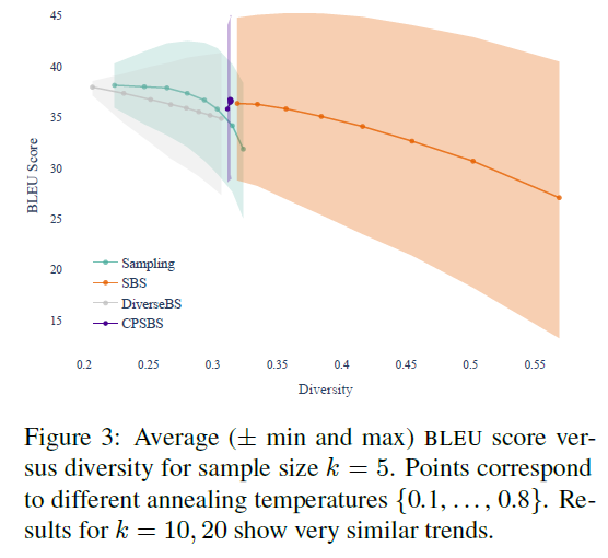
To test the diversity of the sampled translations $Y_T\sim P$, where $w_n=p(\textbf{y}_{\leq t}^{(n)})/(1-p(\textbf{y}_{\leq t}^{(n)}))$ at each time-step $t$ as suggested, an $n$-gram diversity metric is proposed: $D=\sum_{n=1}^{4} \frac{\text{#unique}\,\text{n-grams}\,in\,\text{K}\,\text{strings}}{\text{#}\,\text{n-grams}\,in\,\text{K}\,\text{strings}}$ and three decoding strategy: SBS, DiverseBS and ancestral sampling are compared with CPSBS, results are as follows:
Decoding time evaluation:
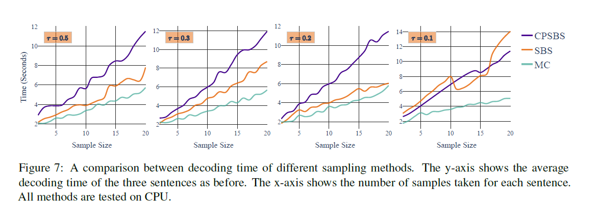
By setting different temperature and sample size, the decoding time for CPSBS, SBS and MC are evaluated:
Enjoy Reading This Article?
Here are some more articles you might like to read next:
