Treasure Hunting 1
Bird’s Eye: Probing for Linguistic Graph Structures with a Simple Information-Theoretic Approach
Here I’m going to present you the first episode of my ‘Treasure Hunting’ series, unlike the ‘Paper Summary’ series, in which a group of papers will be roughly analyzed based on main ideas and motivations. In this series, one paper will be deeply analyzed at a time, focusing not only on the main idea, motivation, shining points but also the writing skills, experimental results etc.
Today I’m going to introduce the paper ‘Bird’s Eye: Probing for Linguistic Graph Structures with a Simple Information-Theoretic Approach’ by Yifan Hou and Mrinmaya Sachan, you can find the paper [here]
Note that: ‘xxx’ means quoted from the paper; xxx is to underline; sub_title is the sub title I named to help understand the structure of the paper; ‘xxx’ is the question / comments I raised to help understand the idea/logic of the paper;
Abstract
- Where dose the ‘graph’ come from ?
The author in this section first introduce us that ‘history of representing our prior understanding of language in the form of graphs’ is ‘rich’, indicating that ‘graph’ can be a useful tool to present a sentence, with this idea bear in mind, it’s then natural to ask that $\longrightarrow$ ‘How much of the information presented by the graph is encoded by a model? (e.g., the word embedding)’.
- What dose ‘probe’ mean ?
And this question actually serves as the motivation of the probing filed of NLP $\longrightarrow$ which is to determine how much information (e.g., syntactic, semantic, which can be represented by graphs ) is learnt by the model. And as how intuition goes, the more information encoded, the better the model. Thus, finding a good, stable probing method that can provide interpretation to the existing models is very important.
- Why we need information theory based probe model ?
However, the previous work is to train a probe model, say, based on accuracy (see Probe model based on training for accuracy for a detailed explanation), which is very unstable (see the discussion in xxx), thus, a probing model based on detecting mutual information between the graph and the embeddings of the to-be-detected model, which can preform steadily, is proposed by the authors.
- What can the proposed model do ?
From a ‘Bird’s Eye’, the model can detect the encoded information for a complete sentence (e.g., the syntactic/semantic information of ‘I like the sunny weather today !’). From a ‘Worm’s Eye’, the model can detect the encoded information for a sub part of the sentence (e.g., the syntactic/semantic information of ‘the sunny weather’).
Introduction
- Background
Graphs are used in many NLP areas and is able to present language structure and its meaning. And there’re probe methods aiming to understand how much information is encoded by pre-trained models
For existing methods, for example: the ‘structural probe’, is a method applying a linear transformation to predict the features (e.g., distance between two words, depth of a word) of a paring tree. However it fails to answer the question $\longrightarrow$ ‘Dose the pre-trained model encode the entire graph ?’ (since it only predicts some features of the parsing tree) and is only applicable to trees instead of general graphs. Moreover, a probe model based on training the accuracy is under the concern that it is trying to solve the task to improve acc instead of doing probing.
- Proposed method
For ‘Bird’s Eye’, the graph (adjacency matrix) is first converted into graph embeddings ($z_1,z_2,z_3,z_4$), and then the mutual information between graph embeddings ($z_1,z_2,z_3,z_4$) and word representations ($x_1,x_2,x_3,x_4$) is calculated by the model, which is the probe results of the to-be-probed model. For ‘Worm’s Eye’, the calculation process is quite like that of the ‘Bird’s Eye’, except for the following difference: ‘Worm’s Eye’ probes the local structure and ‘Bird’s Eye’ probes the entire structure.

Bird’s Eye Probe
- Assumption
By calculating the Mutual Information (MI) $I(\mathcal{X};\mathcal{G})$, where $\mathcal{X}$ is the sentence embeddings (e.g., $n \times d$, for which there’re $n$ words in the sentence, and the embedding dimension for each word is $d$ ), and $\mathcal{G}$ is the corresponding graph structure of that sentence. There’s an assumption about the alignment of words in $\mathcal{X}$ and $\mathcal{G}$ $\longrightarrow$ e.g., the #1 node in $\mathcal{G}$ is the #1 word in the sentence (see here). And for graphs having inconsistent number of words (usually smaller than) with the sentence, ‘an aligner might be needed in some cases (Banarescu et al., 2013).’
- Challenges
-
it’s hard to estimate MI between discrete graphs (e.g., $\mathcal{G}$ which is an discrete adjacency matrix) and continuous features (e.g., $\mathcal{X}$ which is with continuous embeddings), since there’s no unified definition of the MI between them.
-
MI estimation for large sample sizes or high dimensions don’t scale well.
-
same MI values don’t imply same information encoded, e.g., if $I(\mathcal{X};\mathcal{G})=I(\mathcal{X};\mathcal{G~’})$ and $H(\mathcal{G})\neq H(\mathcal{G~’})$, where $G$ is the syntactic tree and $\mathcal{G~’}$ is the semantic graph. Though the MI values are the same, the uncertainty of the two graphs are different, thus it’s hard to simply say that information from the two graphs (which are formed by different mechanisms) has been equally encoded. (e.g., the #1, #3 words from $\mathcal{G}$ are well encoded and #4 word from $\mathcal{G~’}$ may be well encoded)
- Why and How the graph embedding is done ?
Why the adjacency matrix (e.g. $n \times n$) needs to be converted to graph embedding (e.g., $n \times d$) ? It’s because that the adjacency matrix is discrete (no unified definition about MI between discrete and continuous variables) and sparse (computationally wasting), thus a new representation for the graph (i.e., graph embedding) should be computed. And How the graph embedding is computed ? In this paper, the authors used DeepWalk + skip-gram (input: one-hot vector $\mathbb1_v$ for a word, output: continuous vectors $\mathbb1_{v~’}$ for neighboring words), and to get well-learnt graph embeddings, the co-occurrence $L(\theta)$ is to be maximized:
And the graph embeddings ($z_{v_k}$) is later concatenated together, which is
- The math behind the model
Under some conditions (w.r.t. Invariant property of MI), there exists: $\mathcal{G}=f^{-1}(f(\mathcal{G}))$ where $f$ is an invertible function and $\mathcal{Z}=f(\mathcal{G})$. Then the following should hold: $I(\mathcal{X};\mathcal{Z})\approx I(\mathcal{X};\mathcal{G})$, which is the bedrock for converting discrete, sparse adjacency matrix $\mathcal{G}$ to continuous graph embedding $\mathcal{Z}$.
And to estimate $I(\mathcal{X};\mathcal{Z})=KL(\mathbb{P}_{xz}||\mathbb{P}_x\times \mathbb{P}_z)$ under high dimensions, an approximation (see Compression lemma lower bound) is used:
Thus:
And in that sense, the task becomes to find a prefect $T$ that can approximate the real $I(X;Z)=KL(\mathbb{P}_{xz}||\mathbb{P}_x\times \mathbb{P}_z)$ as close as possible based on $\underset {T\in\mathcal{F}}{sup}\,\mathbb{E_{\mathbb{P}_xz}}[T]-log(\mathbb{E_{\mathbb{P}_x\times\mathbb{P}_z}}[e^T])$. And the objective function of which is: (where $T$ is simply a MLP)
Where ${\mathbb{P}_{xz}^{(n)}}$, ${\mathbb{P}_{x}^{(n)}}$ and ${\mathbb{P}_{z}^{(n)}}$ are empirical joint, marginal distributions over a sample, which contains $n$ pairs of (sentence, graph). And for detailed training progress, see in How the estimator is trained.
- Solution to challenge 3
To make the estimated MI value more general and not being affected by the entropy of the graph, the formalism of the graph etc. Two control bounds $I(\mathcal{R};\mathcal{Z})$, $I(\mathcal{Z};\mathcal{Z})$ are introduced to map the MI value $I(\mathcal{X};\mathcal{Z})$ to $[0, 1]$, where $I(\mathcal{R};\mathcal{Z})\leq I(\mathcal{X};\mathcal{Z})\leq I(\mathcal{Z};\mathcal{Z})$, and the relative MI value for $I(\mathcal{X};\mathcal{Z})$ is:
where the $\hat{I}(..;..)$ is the estimate from the model, $\mathcal{R}$ is a random variable independent of the graph $\mathcal{G}$ , and $\hat{I}(\mathcal{Z};\mathcal{Z})$ is actually calculated as $\hat{I}(\mathcal{Z+\epsilon};\mathcal{Z})$ where $\epsilon$ is the noise added to $\mathcal{Z}$ to prevent $\hat{I}(\mathcal{Z};\mathcal{Z})$ from going to infinity.
And by scaling $I(\mathcal{X};\mathcal{Z})$ to $[0, 1]$, the gap between $KL(\mathbb{P}_{xz}||\mathbb{P}_x\times \mathbb{P}_z)$ and $\underset {T\in\mathcal{F}}{sup}\,\mathbb{E_{\mathbb{P}_xz}}[T]-log(\mathbb{E_{\mathbb{P}_x\times\mathbb{P}_z}}[e^T])$ is reduced, since for $(\mathcal{R}, \mathcal{Z})$, the gap is $I(\mathcal{R},\mathcal{Z})-\hat{I}(\mathcal{R},\mathcal{Z})=-\hat{I}(\mathcal{R},\mathcal{Z})$, and by scaling, this ‘gap’ is subtracted from $\hat{I}(\mathcal{X},\mathcal{Z})$ and $\hat{I}(\mathcal{Z},\mathcal{Z})$. Thus, reducing the error brought during training the MLP to approximate function $T$.
- Worm’s Eye probe for local structure
The MI estimate for the local structure $\mathcal{G_s}$ is calculated as:
Where $\mathcal{G_s}={V_s, E_s}$, for all the nodes in $V_s$ of the sub-graph $\mathcal{G_s}$, a noise (kept the same) is added to corresponding embedding $z_s$. Thus a corrupted graph embedding $\mathcal{Z^{‘}}$ is obtained with the to-be-tested local structure masked (noise added). By calculating the MI estimate for the corrupted graph embedding $\mathcal{Z^{‘}}$, it tells us how much the graph without the local structure $\mathcal{G_s}$ has in common with the embedding $\mathcal{X}$, and one minus that tells us how much the local structure $\mathcal{G_s}$ has in common with the embedding $\mathcal{X}$.
Probing for Syntactic and Semantic Graph Structures
For syntactic graph, the Stanford dependency syntax tree is used, and the direction of the edges, the labels (e.g., SUBJ, ATTR etc.) are ignored. And AMR (Abstract Meaning Representation) is used for semantic graph, and an off-the-shelf aligner (see paper [here]) is used for possible situations when there’s no 1-to-1 relation between nodes and words. The direction of edges, labels are ignored as well.
Experiment
- Two things to do in experiments
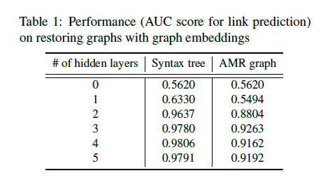
To test the performance and effectiveness of the MI based model, there’ re two things to do: 1. To test the assumption of $I(\mathcal{X};\mathcal{Z})\approx I(\mathcal{X};\mathcal{G})$. Which is to see if $\mathcal{Z} \in \mathbb{R}^{n\times d}$ can be transformed back to $\mathcal{G} \in\mathbb{R}^{n\times n}$, if so, it can be said that the information in $\mathcal{Z}$ can well cover the information in $\mathcal{G}$, thus proving the foundation of the model is right (since without it we won’t be able to compute the MI between discrete and continuous variables); 2. To use the trained probe to detect how much syntactic / semantic information (presented by graphs) is encoded by the pre-trained models (with contextual information), to contrast, the static embeddings (without contextual information) like GloVe is used.
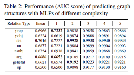
Given two nodes $(v_n, v_m)$, whose graph embeddings are $(z_{v_n},z_{v_m})$. These embeddings are concatenated then fed into the MLP to predict whether there is a link (edge) between $(v_n, v_m)$ or not. After all $n$ nodes’ links are predicted, the AUC score is calculated to show the effectiveness of the graph embedding. Different levels of MLP is used as well, and ‘0’ means linear transformation.
- Probe the entire structure
To probe the syntactic and semantic information encoded in the embeddings, the $MIG$ score is reported.
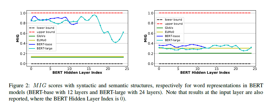
And generally, non-contextual embeddings (GloVe, ELMo-0) perform worse on both syntax and semantics compared with contextual embeddings (Bert-base, Bert-large), and the gap between them on semantic information (right sub-figure) is smaller compared with that of syntactic information (left sub-figure). In that sense, none of them seems to be capable of capturing the semantic information well.
- Probe local structure
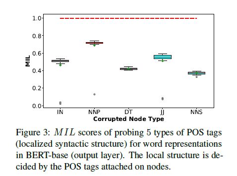
Probe the POS information in PTB (Penn Treebank dataset): POS relations are node labels and the following 5 POS tags are probed: $IN,\,NNP,\,DT,\,JJ,\,NNS$. Corresponding to-be-probed node’s graph embedding is added with a noise consistent with other tags., and the $MIL$ score is reported. ($NNP$: singular proper nouns, $JJ$: adjectives, $NNS$: plural nouns)
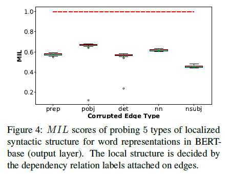
Probe the universal dependency relations in PTB (Penn Treebank dataset): the universal dependency relations in PTB is similar to that of the POS, and $prep,\,pobj,\,det,\,nn,\,nsubj$ are probed with the same method (adding a consistent noise to corresponding graph embedding). ($prep$: prepositional modifiers, $pobj$: object of a preposition, $nn$: noun compound modifier, $nsubj$: nominal subject)
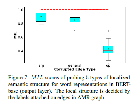
Probe the semantics in AMR graph: There’re 3 relations to be probed: $arg,\,general,\,op$, and the corresponding graph embeddings are corrupted with 50% noise. (since the total 6 relations of AMR are not evenly distributed). The $MIL$ scores are reported as follows:
- Probe using model based on accuracy
To contrast with the MI based probing model, based on the arguments in structural probe (see in Probe model based on training for accuracy), that ‘powerful models such as Bert will easily capture the syntactic and semantic information, thus a simple probing model should be designed’, the authors also trained a acc-based probe model. However, note in here, a simple linear transformation could not even restore the original graph structure from the graph embeddings, suggesting the effectiveness of a simple acc-based probe model (e.g., MLP) may have problems probing. And for probing the entire structure based on an accuracy model:
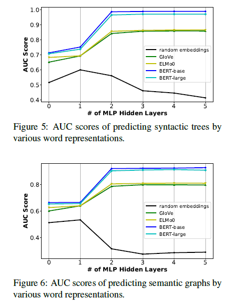
We can see that probing model based on accuracy highly rely on the model’s structure (in this case, number of hidden layers), leading to inconsistency about the probing results. (which calls back to the previous discussion about the drawbacks of acc-based probe model). And for probing the local structure using the acc-based model, similar results can be observed. (Note that the model is first trained to probe the entire structure on training set, then AUC score for each relation is calculated based on the results from test set, and there’s no noise add. For a perturbation setting, refer to A perturbation setting for acc-based probe)
- Discussion about the hyperparameter along with efficiency
Deeper MLPs (used for modeling the function $T$) can achieve tighter lower bound thus having a better estimation of the MI value, meanwhile ‘less efficient than shallow ones. Thus the selection of MI estimator’s complexity is a tradeoff.’ And for potential users, the authors mentioned that can use different graph embedding ways (get better graph embedding), or use sampling strategy (get better MI estimator) to achieve possible precision improvements.
Related work
Mainly introduced the concept of probing: ‘Syntax and Semantics Probing’ and then probing using information theory: ‘Information Theoretic Probe’ and how to estimate mutual information: ‘Mutual Information Estimation’.
Limitations and Future work
The limitations for the work, analyzed by the authors, are two: ‘First, a graph embedding is used, and some structure information could be lost in this process.’, ‘Second, training a MI estimation model is difficult.’. And the authors suggest that future work can be done based on this (graph embedding + MI estimator) framework, exploring methods towards better graph embeddings or MI estimation. And the authors also consider the importance of probing, which may serve as detecting sensitive contents, and helps to deploy neural networks in a better way by gaining syntactic and semantic interpretations for the model.
Writing skill analysis:
I personally quite enjoy the writing style in this paper, first all, it has a very clear Abstract which gives a explicit explanation about e.g., ‘what is probe?’, ‘why we’re doing probe?’, and points out the drawbacks of the existing methods (using ‘However’). And apart from the well-organized Abstract, the authors have the intention to do ‘callbacks’, e.g.: in 2.2 Mutual Information Estimation, they wrote: ‘our objective of the neural network is to find an optimal function in $\mathcal{F}$ and estimate MI, rather than use prediction accuracy. Besides, the neural network is very simple (MLP).’ ,which not only highlighted the simplicity of the proposed method but also again, implied the drawbacks of previous models (‘use prediction accuracy’). Which is an important technique to use in writings.
Shining points and Drawbacks:
Shining points:
First of all, the idea behind this work is quite interesting, which tackles the problem of ‘acc-based probe model may probe based on the complexity of the model instead of the structure’, and by proposing the MI-based probe model, there’re following solutions to solve the problems. Logically, the writing is fluent and reasonable.
Also, the proposed framework is flexible and serves the motivations well, by firstly encoding sparse adjacency matrix into continuous graph embedding, which together with the continuous word embeddings will be used to compute the MI. ($\longrightarrow$ solves the problem that it’s unclear to compute the MI between discrete and continuous variables) And later the compression lower bound is used to approximate the MI between graph and word embeddings, which can be modeled by a MLP. ($\longrightarrow$ solves the problem of estimating MI). And two control bounds are used to map the MI value between [0, 1]. ($\longrightarrow$ solves the problem of standalone MI value may unable to reflect information encoded)
Last but not least, the way how the authors proposed to probe the local structure is also novel, which corrupts corresponding graph embeddings, and then calculate the relative MI that is mapped to [0, 1], which indicates how much information except for the to-be-probed local structure is encoded, thus, one minus that will be the MI for the local structure.
Drawbacks:
The first drawback I think is the graph embedding algorithms, since the authors point out that the previous acc-based probe models rely on its complexity instead of the graph structure, and MLPs of different layers are used to prove this, I think the authors should show the results of different graph embedding algorithms (and of course I think different graph embedding algorithms will result different MI estimations), and show that the performance is not easily affected.
The second one I think is about the assumption made when trying to convert discrete adjacency matrix $\mathcal{G}\in\mathbb{R}^{n\times n}$ to continuous graph embedding $\mathcal{Z}\in\mathbb{R}^{n\times d}$, which is: $I(\mathcal{X};\mathcal{Z})\approx I(\mathcal{X};\mathcal{G})$. However, if look carefully into the Invariant property of MI, you will see that if $\mathcal{G}$ and $\mathcal{Z}$ are homeomorphic, the following should hold: $I(\mathcal{X};\mathcal{Z})= I(\mathcal{X};\mathcal{G})$, and in this case $\mathcal{G}$ is actually in $\mathbb{R}^{n}$ while $\mathcal{Z}$ is actually in $\mathbb{R}^{d}$, which by dimension, are impossible to be homeomorphic. One explanation is that this is the reason why the authors used ‘$\approx$’’ instead of ‘$=$’ , however, in this sense, it’s hard to know whether it holds mathematically or holds engineeringly. Another explanation is that if we assume that there exists a gold graph embedding $\mathcal{Z}_g\in\mathbb{R}^{n\times d}$ , which can be constructed from the discrete adjacency matrix $\mathcal{G}$ , and $\mathcal{Z}_g$ includes every information stored in $\mathcal{G}$ , thus, the way of doing graph embedding $\mathcal{Z}\in\mathbb{R}^{n\times d}$ out of $\mathcal{G}$ is just the mimicking of $\mathcal{Z}_g$ , for which is in the same space $\mathbb{R}^{d}$ with $\mathcal{Z}_g$ . Thus, $\mathcal{Z}$ and $\mathcal{Z}_g$ can be homeomorphic, and the Invariant property of MI may hold. However, this still raise another question, dose the gold $\mathcal{Z}_g$ exist ? ( although the authors did the restoring experiment suggesting its existence) and how is it achieved ?
Supplementary
Probe model based on training for accuracy
To gain a clue about the acc-based probe model, I here simply introduce the main methodology of the paper ‘A Structural Probe for Finding Syntax in Word Representations’ [paper], i.e. ‘structural probe’
In this work, the authors assume that if the tree structure of a sentence is encoded, then the square of the L2 distance between embeddings of two words can be linearly transformed into the distance between the same two words in the tree structure. And the following distance can be defined:
where $B\in\mathbb{R}^{k\times m}$ is the linear transformation which is to be learnt during training, $h_k^l$ is the embedding of the $k$-th word in the $l$-th sentence. And the training objective is:
where $|s^l|$ is the length of the sentence.
Also, if the tree structure of a sentence is encoded, the parse depth $||w_i||$ of word $w_i$ can be probed too, and to train the probe model to have an accurate estimation, a new distance is defined as: $||h_i||_A=(Bh_i)^T(Bh_i)$, then $B$ is learnt with a similar training objective to that of distance probe.
This property comes from the paper ‘Estimating Mutual Information’ (see [paper]), where:
If $X^{‘}=F(X)$ and $Y^{‘}=G(Y)$ are homeomorphisms (see more in here) and $J_X=||\partial X/\partial X^{‘}||$, $J_Y=||\partial Y/\partial Y^{‘}||$, then we have:
And thus, by definition: $I(X^{‘},Y^{‘})=\int\int d_{x^{‘}}d_{y^{‘}}\mu^{‘}(x^{‘},y^{‘})log\frac{\mu^{‘}(x^{‘},y^{‘})}{\mu_x^{‘}(x^{‘})\mu_y^{‘}(y^{‘})}=\int\int d_{x}d_{y}\mu(x,y)log\frac{\mu(x,y)}{\mu_x(x)\mu_y(y)}=I(X;Y)$
And for the derivation of $\mu^{‘}(x^{‘},y^{‘})=J_X(x^{‘})J_Y(y^{‘})\mu(x,y)$, please consider the following:
since $X^{‘}=F(X)$ is homeomorphism, thus, we have: $|p(x)\,d_x|=|q(x^{‘})\,d_{x{‘}}|$, the distribution of the new variable $X^{‘}$can be written as: $q(x^{‘})=p(x)|{d_x}/{d_{x^{‘}}}|$, which is called the Jacobian transformation. Similar results can be obtained for joint distributions, where for example, $|{d_x}/{d_{x^{‘}}}|$ becomes $|\partial x/\partial x^{‘}|$.
It’ a continuous function between topological spaces whose reverse is continuous as well. If between two spaces there is a homeomorphism, their topological properties are preserved during the mapping. There some examples: 1. open interval $(a, b), a\lt b$ is homeomorphic to real numbers $\mathbb{R}$; 2. $\mathbb{R}^m,\mathbb{R}^n$ are not homeomorphic if $m\neq n$. For more information, please refer to [wiki]
This bound is derived from ‘On Bayesian bounds’ (see [paper])
First of all, let $\mathcal{H}$ be the set of predictors under consideration, and $h$ is one of them. Further define that $\phi(h)$ is any measurable function on $\mathcal{H}$, $P$ and $Q$ are any distributions on $\mathcal{H}$. Then we have:
For (1) we have:
Where the ‘$\leq$’ comes from Jensen’s inequality. (For concave it’s the reverse version of the normally known $f(E[X])\leq E[f(X)]$, for $f$ is a convex function)
For (2), just simply let $\phi(h)=log(\frac{dQ(h)}{dP(h)})$, then it achieves the upper bound, thus:
For the training objective: $\underset {\theta\in\Theta}{max}(\,\mathbb{E_{\mathbb{P}_xz^{(n)}}}[T_\theta]-log(\mathbb{E_{\mathbb{P}_x^{(n)}\times\mathbb{P}_z^{(n)}}}[e^{T_\theta}]))$, there’re two terms to be optimized: one is the joint distribution term: $\mathbb{E_{\mathbb{P}_xz^{(n)}}}[T_\theta]$ , the other is the marginal distribution term: $log(\mathbb{E_{\mathbb{P}_x^{(n)}\times\mathbb{P}_z^{(n)}}}[e^{T_\theta}])$ .
And for the joint distribution term, the word representation $\mathcal{X}$ is concatenated with the graph embedding $\mathcal{Z}$, and then put into the MLP to compute a scalar (see here), then average of scalars is computed as the expectation $\mathbb{E_{\mathbb{P}_xz^{(n)}}}[T_\theta]$.
For the marginal distribution term, the representation $\mathcal{X}$ is randomly shuffled and then concatenated with the graph embedding $\mathcal{Z}$, and the same MLP is used to compute a scalar for marginal distribution, and then its exponential is taken and the average of the exponentials is computed as the expectation $\mathbb{E_{\mathbb{P}_x^{(n)}\times\mathbb{P}_z^{(n)}}}[e^{T_\theta}]$.
How the scalar for one sentence is computed
For one sentence, say with 10 words, its word presentation $\mathcal{X}\in\mathbb{R}^{10\times 768}$, where 768 is the hidden size of each word, and its graph embedding $\mathcal{Z}\in\mathbb{R}^{10\times 128}$, where 128 is the embedding size of each node (indicating corresponding word), they are encoded into the same space with a dimension of 32: $\mathcal{X}\in\mathbb{R}^{10\times 768}$ $\longrightarrow$ $\mathcal{X}^{‘}\in\mathbb{R}^{10\times 32}$, $\mathcal{Z}\in\mathbb{R}^{10\times 128}$ $\longrightarrow$ $\mathcal{Z}^{‘}\in\mathbb{R}^{10\times 32}$, and then $\mathcal{X}^{‘}$ and $\mathcal{Z}^{‘}$ are concatenated to be a representation of $\mathbb{R}^{10 \times 64}$, and this intermediate space is then projected to a scalar, which is to project: $\mathbb{R}^{10 \times 64}$ $\longrightarrow$ $\mathbb{R}^{10 \times 1}$, and the average of the 10 scalars is computed.
A perturbation setting for acc-based probe
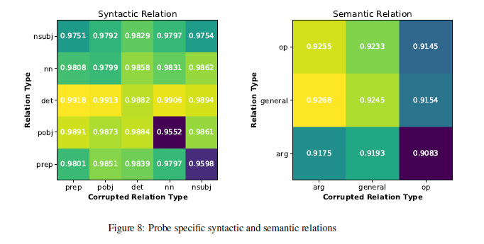
The word embedding is corrupted with the same noise, and for each relation, same amount of words are corrupted. And Worm’s Eye is used to predict the relations with the corrupted word embeddings. The results are as follows:
Enjoy Reading This Article?
Here are some more articles you might like to read next: